Convolutions and Backpropagations
Ever since AlexNet won the ImageNet competition in 2012, Convolutional Neural Networks (CNNs) have become ubiquitous. Starting from the humble LeNet to ResNets to DenseNets, CNNs are everywhere.
But have you ever wondered what happens in a Backward pass of a CNN, especially how Backpropagation works in a CNN. If you have read about Backpropagation, you would have seen how it is implemented in a simple Neural Network with Fully Connected layers. (Andrew Ng’s course on Coursera does a great job of explaining it). But, for the life of me, I couldn’t wrap my head around how Backpropagation works with Convolutional layers.
The more I dug through the articles related to CNNs and Backpropagation, the more confused I got. Explanations were mired in complex derivations and notations and they needed an extra-mathematical muscle to understand it. And I was getting nowhere.
I know, you don’t have to know the mathematical intricacies of a Backpropagation to implement CNNs. You don’t have to implement them by hand. And hence, most of the Deep Learning Books don’t cover it either.
So when I finally figured it out, I decided to write this article. To simplify and demystify it. Of course, it would be great if you understand the basics of Backpropagation to follow this article.

The most important thing about this article is to show you this:
We all know the forward pass of a Convolutional layer uses Convolutions. But, the backward pass during Backpropagation also uses Convolutions!
So, let us dig in and start with understanding the intuition behind Backpropagation. (And for this, we are going to rely on Andrej Karpathy’s amazing CS231n lecture — https://www.youtube.com/watch?v=i94OvYb6noo).
But if you are already aware of the chain rule in Backpropagation, then you can skip to the next section.
Understanding Chain Rule in Backpropagation:
Consider this equation
f(x,y,z) = (x + y)z
To make it simpler, let us split it into two equations.
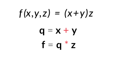
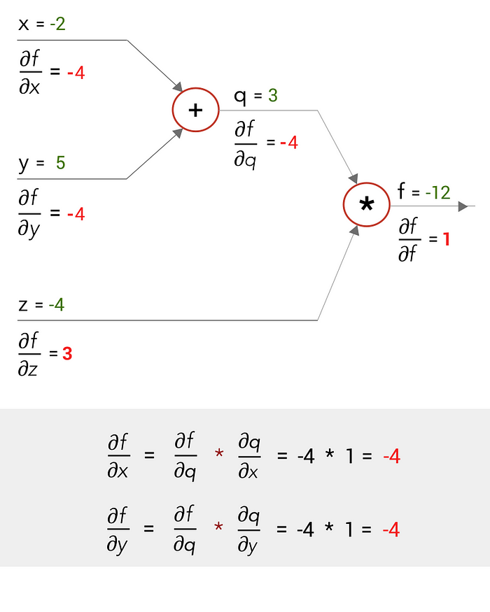
Now, let us draw a computational graph for it with values of x, y, z as x = -2, y = 5, z = 4.

When we solve for the equations, as we move from left to right, (‘the forward pass’), we get an output of f = -12
Now let us do the backward pass. Say, just like in Backpropagations, we derive the gradients moving from right to left at each stage. So, at the end, we have to get the values of the gradients of our inputs x,y and z — ∂f/∂x and ∂f/∂y and ∂f/∂z (differentiating function f in terms of x,y and z)
Working from right to left, at the multiply gate we can differentiate f to get the gradients at q and z — ∂f/∂q and ∂f/∂z . And at the add gate, we can differentiate q to get the gradients at x and y — ∂q/∂x and ∂q/∂y.

We have to find ∂f/∂x and ∂f/∂y but we only have got the values of ∂q/∂x and ∂q/∂y. So, how do we go about it?

This can be done using the chain rule of differentiation. By the chain rule, we can find ∂f/∂x as

And we can calculate ∂f/∂x and ∂f/∂y as:
Chain Rule in a Convolutional Layer
Now that we have worked through a simple computational graph, we can imagine a CNN as a massive computational graph. Let us say we have a gate f in that computational graph with inputs x and y which outputs z.

We can easily compute the local gradients — differentiating z with respect to x and y as ∂z/∂x and ∂z/∂y
For the forward pass, we move across the CNN, moving through its layers and at the end obtain the loss, using the loss function. And when we start to work the loss backwards, layer across layer, we get the gradient of the loss from the previous layer as ∂L/∂z. In order for the loss to be propagated to the other gates, we need to find ∂L/∂x and ∂L/∂y.

The chain rule comes to our help. Using the chain rule we can calculate ∂L/∂x and ∂L/∂y, which would feed the other gates in the extended computational graph

So, what has this got to do with Backpropagation in the Convolutional layer of a CNN?
Now, lets assume the function f is a convolution between Input X and a Filter F. Input X is a 3x3 matrix and Filter F is a 2x2 matrix, as shown below:

Convolution between Input X and Filter F, gives us an output O. This can be represented as:


This gives us the forward pass! Let’s get to the Backward pass. As mentioned earlier, we get the loss gradient with respect to the Output O from the next layer as ∂L/∂O, during Backward pass. And combining with our previous knowledge using Chain rule and Backpropagation we get:

As seen above, we can find the local gradients ∂O/∂X and ∂O/∂F with respect to Output O. And with loss gradient from previous layers — ∂L/∂O and using chain rule, we can calculate ∂L/∂X and ∂L/∂F.
Well, but why do we need to find ∂L/∂X and ∂L/∂F?
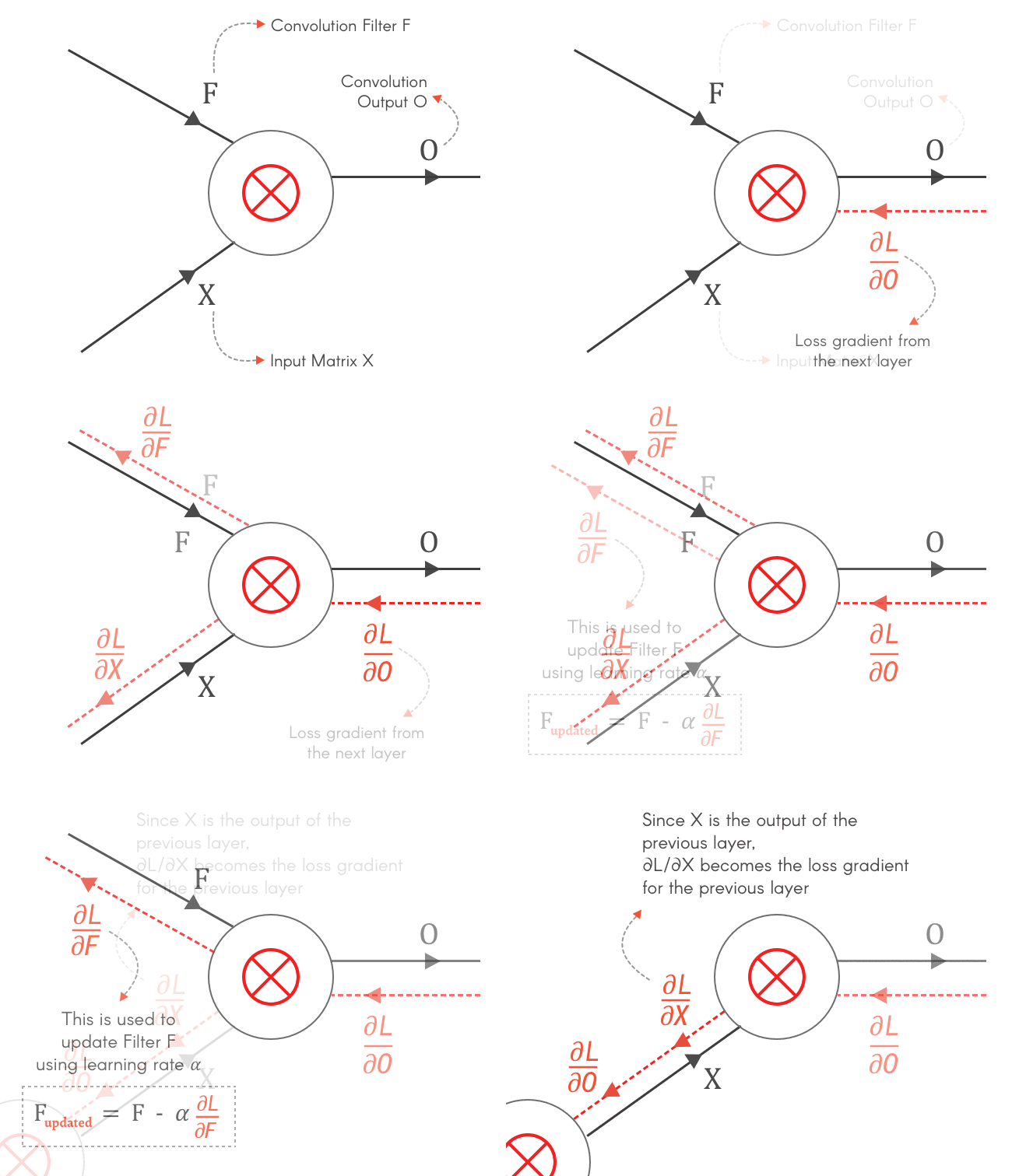
So let’s find the gradients for X and F — ∂L/∂X and ∂L/∂F
Finding ∂L/∂F
This has two steps as we have done earlier.
- Find the local gradient ∂O/∂F
- Find ∂L/∂F using chain rule
Step 1: Finding the local gradient — ∂O/∂F:
This means we have to differentiate Output Matrix O with Filter F. From our convolution operation, we know the values. So let us start differentiating the first element of O- O¹¹ with respect to the elements of F — F¹¹ , F¹², F²¹ and F²²

Step 2: Using the Chain rule:
As described in our previous examples, we need to find ∂L/∂F as:

O and F are matrices. And ∂O/∂F will be a partial derivative of a matrix O with respect to a matrix F! On top of it we have to use the chain rule. This does look complicated but thankfully we can use the formula below to expand it.

Expanding, we get..
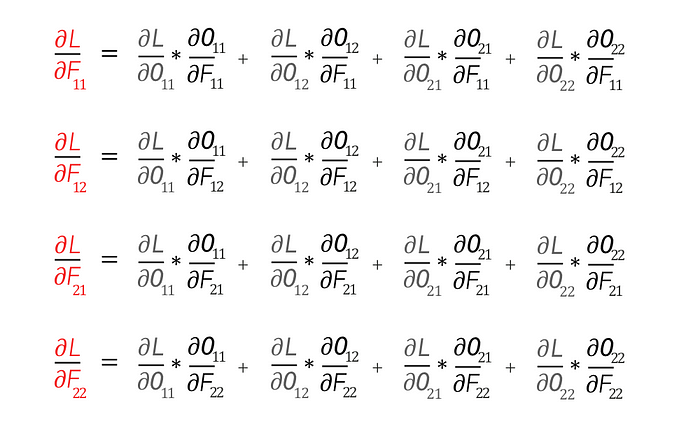
Substituting the values of the local gradient — ∂O/∂F from Equation A, we get

If you closely look at it, this represents an operation we are quite familiar with. We can represent it as a convolution operation between input X and loss gradient ∂L/∂O as shown below:

∂L/∂F is nothing but the convolution between Input X and Loss Gradient from the next layer ∂L/∂O
Finding ∂L/∂X:
Step 1: Finding the local gradient — ∂O/∂X:
Similar to how we found the local gradients earlier, we can find ∂O/∂X as:

Step 2: Using the Chain rule:

Expanding this and substituting from Equation B, we get

Ok. Now we have the values of ∂L/∂X.
Believe it or not, even this can be represented as a convolution operation.
∂L/∂X can be represented as ‘full’ convolution between a 180-degree rotated Filter F and loss gradient ∂L/∂O
First, let us rotate the Filter F by 180 degrees. This is done by flipping it first vertically and then horizontally.

Now, let us do a ‘full’ convolution between this flipped Filter F and ∂L/∂O, which can be visualized as below: (It is like sliding one matrix over another from right to left, bottom to top)
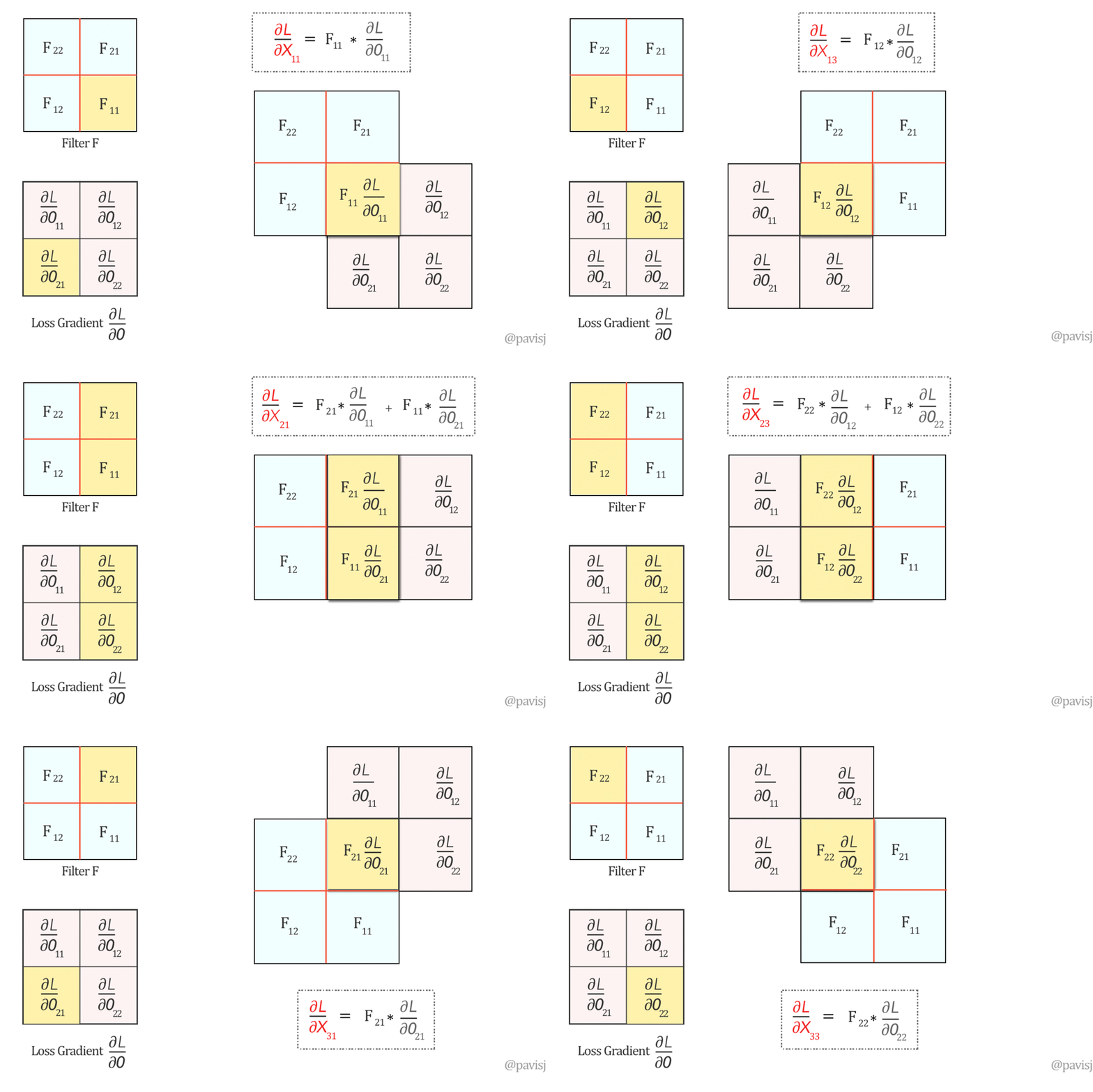
The full convolution above generates the values of ∂L/∂X and hence we can represent ∂L/∂X as
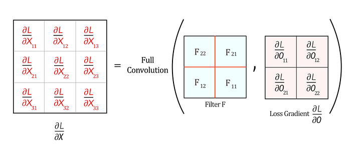
Well, now that we have found ∂L/∂X and ∂L/∂F, we can now come to this conclusion
Both the Forward pass and the Backpropagation of a Convolutional layer are Convolutions
Summing it up:

Hope this helped to explain how Backpropagation works in a Convolutional layer of a CNN.
If you want to read more about it, do look at these links below. And do show some love by clapping for this article. Adios! :)
